Data & figures — the endpoints, and the plots built from them

A Three REST resources

Since August 2026 the source data are published as REST resources rather than reached only through a PostgreSQL connection. They are public: no key, no account, no VPN. That is what makes the datings reproducible by someone outside the project.

https://www1.rgzm.de/rest/samianresearch/datedsites — the input

One record per dated stamp: findspot, potter, die, and the potter's date range. These are the same rows sql/v_ips_dated_stamps.sql delivers, and the model is computed from them. Currently 1391 records.

https://www1.rgzm.de/rest/samianresearch/datedsitesstatistics — the output

One row per findspot, everything already aggregated: the interval, both quality axes, σ, k and the model parameters. This is the model's result, computed in the database, and it is what py/ips_model.py is measured against. Currently 40 rows and 41 columns.

https://www1.rgzm.de/ips/lod/ips_stamps.csv — a listing, not an input

Pipe-delimited CSV of the stamp list: site, findspot, potter, die, stamp number — and no dates. Useful for looking things up, unusable as model input, because the model needs datemin and datemax per stamp. This was tried first and produced an empty model in silence, which is why it is written down rather than discovered again.

What the payloads actually look like

Both REST resources answer with ColdFusion's query serialisation: a COLUMNS list and a DATA list of positional rows — not a list of objects. Column names are upper case; everything else in the project uses lower case.

{ "records": 1391,
  "success": true,
  "data": {
    "COLUMNS": ["THE_ID", "THE_SITE", "THE_FINDSPOT", …, "DATEMIN", "DATEMAX"],
    "DATA": [ [1000136, "London", "New Fresh Wharf: quay", …, 200, 260],
               … ] } }

The statistics format is not fixed. It has been served as pipe-delimited CSV and, from the live endpoint, as the ColdFusion serialisation above. load_statistics() in py/ips_rest.py accepts either, plus a plain JSON array, and reports what it received when it can make sense of none of them. The pipe-delimited variant also renders SQL NULL as an empty field — indistinguishable from an empty string — and omitted two columns the database query produces, the_id and q_repetition. A comparison that assumes the two column sets match will report dozens of differences that are not there.

B Fetching them

Nothing beyond a browser is needed to look; the pipeline uses urllib from the standard library, so there is no dependency and no credential anywhere in the code.

# look at it
curl -s https://www1.rgzm.de/rest/samianresearch/datedsites | head -c 400

# save both payloads where the pipeline expects them
curl -s -o data/source/datedsites.json \
     https://www1.rgzm.de/rest/samianresearch/datedsites
curl -s -o data/source/datedsitesstatistics.csv \
     https://www1.rgzm.de/rest/samianresearch/datedsitesstatistics

# or from Python, through the project's own reader
import sys; sys.path.insert(0, "py")
import ips_rest
from pathlib import Path

paths, origin, notes = ips_rest.resolve(Path("data/source"))
rows = ips_rest.load_datedsites_json(paths["datedsites"])
print(origin, len(rows))        # -> live 1391

Live first, archive as fallback. resolve() tries the endpoints and falls back to the copies in data/source/ only when they cannot be reached. That order is deliberate: a stale export is the failure this project has actually suffered — the whole corpus was once rebuilt from a file carrying the wrong t0, and the Böckleareal findspots went missing for a week without anyone noticing. Partial success counts as failure: if only one of the two payloads arrives, both are read from the archive, because checking a fresh stamp list against a stale reference would make the disagreement look like a defect in the model.

Reproducibility is preserved rather than traded away. What was fetched is written into data/source/ and stamped into data/SNAPSHOT.json with the date, byte sizes and SHA-256 of each payload, the record counts and the model parameters in force. A build from the archive alone produces the same figures — it just says which of the two it did. Cite the snapshot as the data state rather than asserting a fixed number of findspots: Samian Research is a live database.

Invocation	Reads
python py/main.py	the endpoints, falling back to `data/source/`
python py/main.py --offline	`data/source/` only, no network attempt — what CI runs
python py/main.py --no-rest	the CSV in `data/` as it stands; reproduces an older build exactly
python py/main.py --csv data/other.csv	a named export instead

C The figures

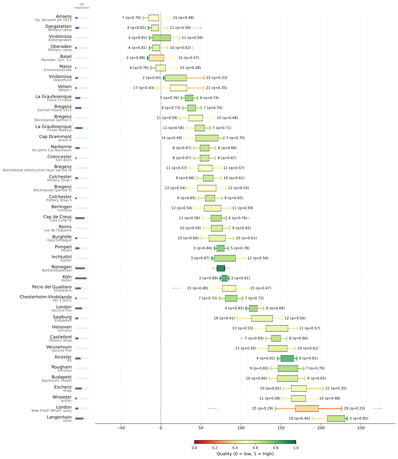
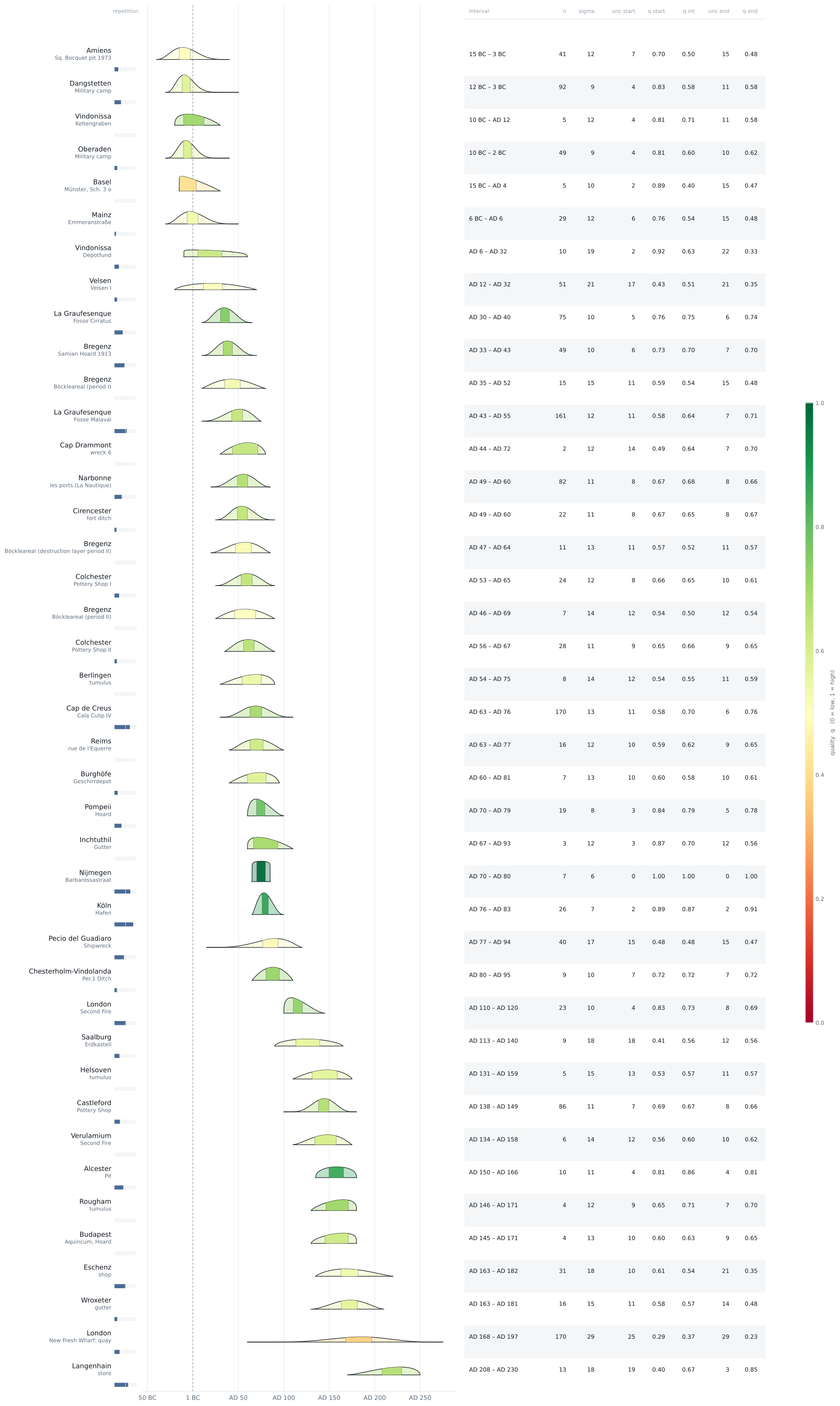
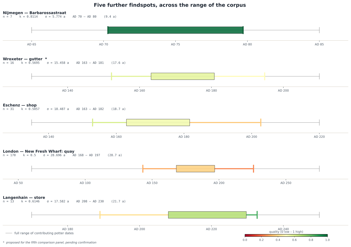
Five sheets, all written by python py/main.py into img/, each as SVG and as JPG at 300 dpi. They are generated from the same rows as the interactive plot, so a figure cannot disagree with the table beside it.

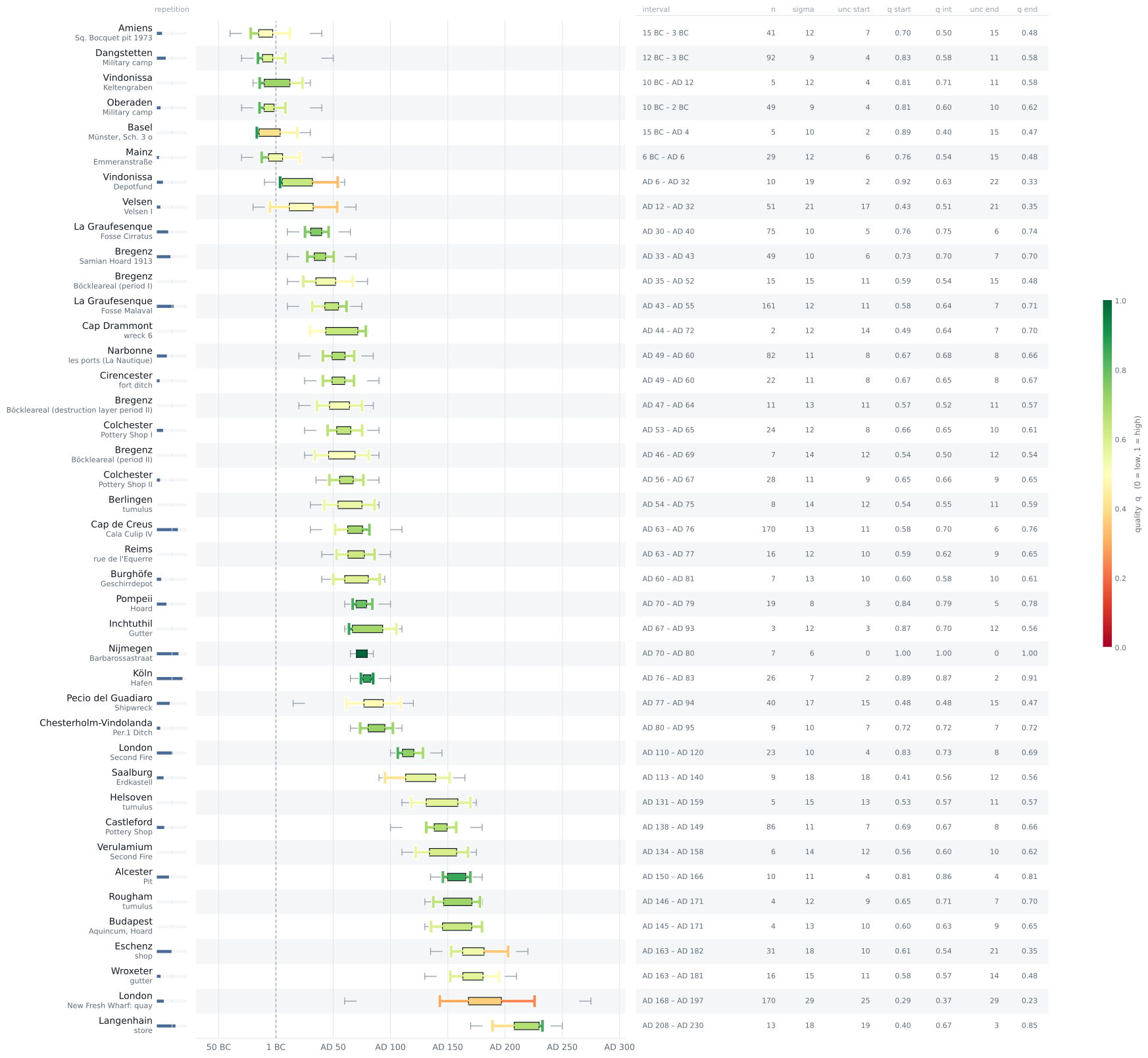
All findspots as horizontal intervals, ordered chronologically, with coloured
whiskers and a repetition bar in the left margin — **v2 · modern.** The main figure. Every findspot as one row: the box is the dated interval coloured by `q_interval`, the whiskers carry `q_start` and `q_end` in their own colours, the thin line behind is the full range of the contributing potters, and the bar in the left margin is the second quality axis, `q_repetition`. The encoding is identical to the web plot; only the setting is different — typography, a quieter grid, a BC/AD axis, a value table. SVG, 376 kB · JPG, 300 dpi, 1.8 MB

The same intervals in the layout of the original D3 web figure — **v1 · classic.** The D3 web figure one to one: capped whiskers, extreme-value stubs, box edges dashed where an uncertainty exists, the RdYlGn ramp and the gradient legend. Deliberately left untouched so that the web output and the print version stay comparable. SVG, 309 kB · JPG, 300 dpi, 1.4 MB

One density curve per findspot, stacked chronologically — **v2 · gauss.** The same findspots as distributions rather than as boxes: each row is the date distribution its stamps imply, with the areas normalised equal across rows so that the shapes can be compared. The curves are bounded by the extremes of the contributing potters — there are no tails to clip, and none is drawn, because a tail would be a claim the figure is not making. SVG, 1.4 MB · JPG, 300 dpi, 2.3 MB

Five panels, one per reference ensemble, each with a vertical terminus line — **v3 · calibration.** The five ceramic-independent reference ensembles — Dangstetten, Oberaden, Velsen I, Pompeii, Inchtuthil — one panel each, with the independent terminus drawn as a vertical line across the modelled interval. This is the whole calibration argument for τ, made visible rather than asserted: the reader can see for himself whether the line falls inside the box. Each panel carries its own axis, because a shared one would compress Dangstetten's nine-year interval into something narrower than the line drawn for it. SVG, 150 kB · JPG, 300 dpi, 700 kB · what it rests on, §7a

Five further findspots in the same panel layout, without terminus lines — **v3 · findspots.** Five further findspots of archaeological interest, spanning the rest of the range, in the same idiom. No terminus is drawn: these are findspots the model *dates*, not findspots that *test* it. They are kept on their own sheet for that reason — side by side with the references, the five reference panels would read as five ordinary examples among ten and the calibration argument would stop being the point of the figure. SVG, 116 kB · JPG, 300 dpi, 562 kB

D Embedding them elsewhere

The figures on this page are not copies. Each <img> points straight at the file in the repository, so a rebuild that changes a figure changes what this page shows, and there is no second version to keep in step.

<img src="https://raw.githubusercontent.com/leiza-rse/IPSDatedSites/main/img/plot_v2_modern.svg"
     alt="Findspot datings from samian potters' stamps" loading="lazy">

Replace the file name with any of the five. raw.githubusercontent.com serves .svg as image/svg+xml and .jpg as image/jpeg, so both work in an ordinary <img> tag; the path pattern is …/main/img/name.svg|jpg, and pinning a commit hash instead of main freezes the figure at a known state.

Use	Take	Why
web page, this application	.svg	text stays selectable and the figure stays sharp at any zoom
print, a submitted manuscript	.jpg	300 dpi, and no dependency on how a renderer treats fonts in SVG
a slide	.jpg	the large SVGs carry tens of thousands of elements; some presentation software will not thank you

The SVGs are byte-stable. SOURCE_DATE_EPOCH and a fixed svg.hashsalt are set before matplotlib is imported, so a rebuild that changes nothing produces an identical file. Without that, matplotlib writes a fresh timestamp and freshly randomised element identifiers every run, every figure appears modified in git for ever, and a real change to a published figure goes unnoticed among the noise. It also means a figure you embedded and one rebuilt six months later can be compared with cmp.

Do not edit the files in img/. They are build output and the next run overwrites them. Everything the figures show — margins, row height, sort order, colour ramp — is read from the graph and the model parameters, so a change belongs in py/ips_render.py or in the parameters, not in the SVG.

Rebuilding them

python py/main.py                       # everything, figures included
python py/main.py --skip-plots          # everything except the figures
python py/main.py --img-out /tmp/figs   # write them somewhere else
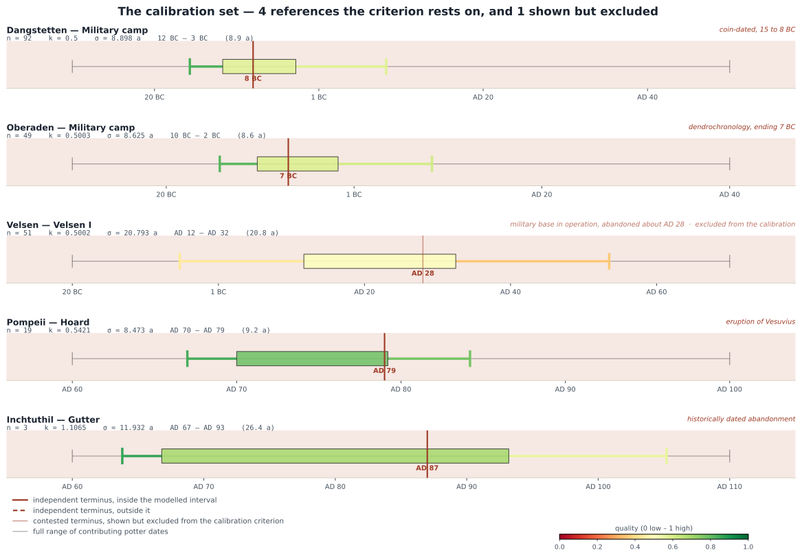
python py/make_calibration_panels.py    # the two v3 panel sheets alone

The panel sheets read the CSV directly rather than the graph, because the calibration argument has to be checkable against the source table without a graph in between. The termini are not restated in the plotting code either: they are read from CALIBRATION_REFERENCES in py/ips_rdf_export.py, which is also what the RDF export publishes as lado:calibratedAgainst. One list, one place to correct.